Text Mining in Python

Libraries and useful links

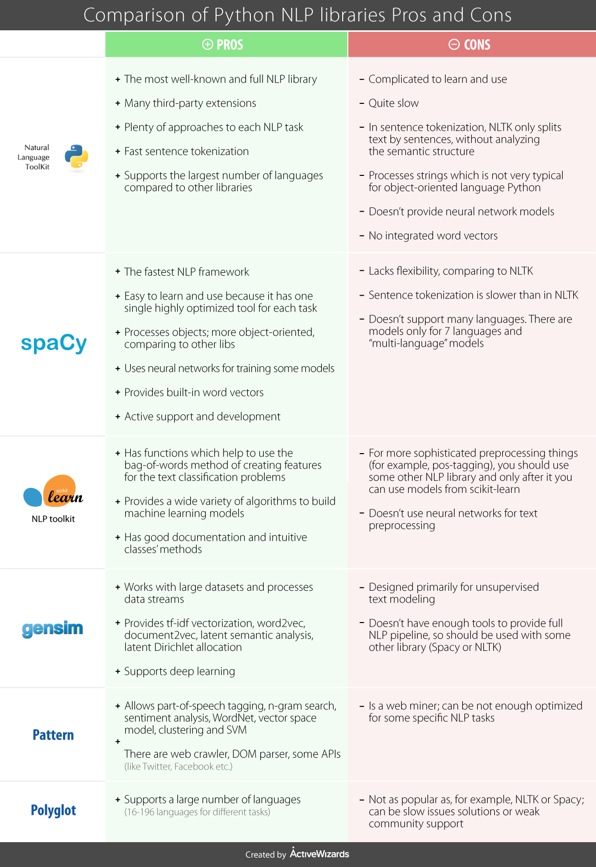
https://www.kdnuggets.com/2018/07/comparison-top-6-python-nlp-libraries.html

How to install NLTK behind proxy:

conda install nltk or pip install –proxy=https://p998phd:p998phd@proxyvip-se.sbcore.net:8080 –trusted-host pypi.python.org -U nltk

then open jupyter notebook:

import nltk
nltk.set_proxy('https://p998phd:p998phd@proxyvip-se.sbcore.net:8080')
nltk.download()

Basic functions

Here are useful functions for cutting a sentence into words, getting the singular form, getting the root of each word:

import string
from nltk.tokenize import RegexpTokenizer

def splitToWords(stringOfWords):
  tokenizer = RegexpTokenizer("[\w']+")
  words = tokenizer.tokenize(stringOfWords)
  words = lower_function(words)
  return words


def lower_function(list_input):
  return [x.lower() for x in list_input]


def lemmatize_function(list_input):
  wordnet_lemmatizer = WordNetLemmatizer()
  return [wordnet_lemmatizer.lemmatize(i) for i in list_input]


def stem_function(list_input):
  snowball_stemmer = SnowballStemmer("english")
  #lancaster_stemmer = LancasterStemmer()
  return [snowball_stemmer.stem(i) for i in list_input]


def remove_stopWords_function(list_input):
  punctuation = list(string.punctuation)
  stop = stopwords.words('english') + punctuation
  return [term for term in list_input if term not in stop]

#INPUT
text = "Nonsense?  kiss off, geek. what I said is true.  I'll have your account terminated."

text = splitToWords(text)                 #tokenizes (=splits in words)
text = remove_stopWords_function(text)    #Removes stopwords ("the",...)
text = lemmatize_function(text)           #Lemmatiz = gets singular form of words when applicable
text = stem_function(text)                #Stemming = keeps root of words only
print(text)

Output: [‘nonsens’, ‘kiss’, ‘geek’, ‘said’, ‘true’, “i’ll”, ‘account’, ‘termin’]

Another useful text cleaning function can be found here:

def standardize_text(df, text_field):
  df[text_field] = df[text_field].str.replace(r"http\S+", "")
  df[text_field] = df[text_field].str.replace(r"http", "")
  df[text_field] = df[text_field].str.replace(r"@\S+", "")
  df[text_field] = df[text_field].str.replace(r"[^A-Za-z0-9(),!?@\'\`\"\_\n]", " ")
  df[text_field] = df[text_field].str.replace(r"@", "at")
  df[text_field] = df[text_field].str.lower()
  return df

questions = standardize_text(df, “text”)

taken from the excellent tutorial on topic classification: https://github.com/hundredblocks/concrete_NLP_tutorial/blob/master/NLP_notebook.ipynb Here for the blog: https://blog.insightdatascience.com/how-to-solve-90-of-nlp-problems-a-step-by-step-guide-fda605278e4e?lipi=urn%3Ali%3Apage%3Ad_flagship3_feed%3BqGDpQk2XQQ2DhR08PHkmqg%3D%3D

Other tokenizing, from DataCamp:

# Import necessary modules
from nltk.tokenize import sent_tokenize
from nltk.tokenize import word_tokenize

# Split scene_one into sentences: sentences
sentences = sent_tokenize(scene_one)

# Use word_tokenize to tokenize the fourth sentence: tokenized_sent
tokenized_sent = word_tokenize(sentences[3])

# Make a set of unique tokens in the entire scene: unique_tokens
unique_tokens = set(word_tokenize(scene_one))

# Print the unique tokens result
print(unique_tokens)

Intro to regular expressions (REGEX)

Examples of regex patterns:

pattern1 = r”#w+” This says that we want to catch terms like ‘#thing’

pattern2 = r”([#|@]w+)” This says that we want to catch terms like ‘#thing’ or ‘@thing’

Let’s say we have some german text like this:

german_text = ‘Wann gehen wir zum Pizza? 🍕 Und fährst du mit Über? 🚕’

1. We want to tokenize all words: all_words = word_tokenize(german_text) print(all_words) Output: [‘Wann’, ‘gehen’, ‘wir’, ‘zum’, ‘Pizza’, ‘?’, ‘🍕’, ‘Und’, ‘fährst’, ‘du’, ‘mit’, ‘Über’, ‘?’, ‘🚕’]

2. We want all words starting by a capital letter (including Ü!!!) capital_words = r”[A-ZÜ]w+” print(regexp_tokenize(german_text,capital_words)) Output: [‘Wann’, ‘Pizza’, ‘Und’, ‘Über’]

3. We want all symbols! For that we can use the list of them in the pattern: # Tokenize and print only emoji emoji = “[’U0001F300-U0001F5FF’|’U0001F600-U0001F64F’|’U0001F680-U0001F6FF’|’u2600-u26FFu2700-u27BF’]” print(regexp_tokenize(german_text,emoji)) Output: [’🍕’, ‘🚕’]

So in theory we can capture anything.

Bag of Words (BOW)

The most primitive method. The bag-of-words is a representation of text that describes the occurrence of words within a document. It involves two things:

A vocabulary of known words.
A measure of the presence of known words.

Why is it is called a “bag” of words? That is because any information about the order or structure of words in the document is discarded and the model is only concerned with whether the known words occur in the document, not where they occur in the document.

The intuition behind the Bag of Words is that documents are similar if they have similar content. Also, we can learn something about the meaning of the document from its content alone.

For example, if our dictionary contains the words {Learning, is, the, not, great}, and we want to vectorize the text “Learning is great”, we would have the following vector: (1, 1, 0, 0, 1).

A problem with the Bag of Words approach is that highly frequent words start to dominate in the document (e.g. larger score), but may not contain as much “informational content”. Also, it will give more weight to longer documents than shorter documents.

TF-IDF (Term Frequency - Inverse Document Frequency)

A very good intro to TF-IDF: https://janav.wordpress.com/2013/10/27/tf-idf-and-cosine-similarity/

One approach is to rescale the frequency of words by how often they appear in all documents so that the scores for frequent words like “the” that are also frequent across all documents are penalized. This approach to scoring is called Term Frequency-Inverse Document Frequency, or TF-IDF for short, where:

Term Frequency: is a scoring of the frequency of the word in the current document.

TF = (Number of times term t appears in a document)/(Number of terms in the document)

Inverse Document Frequency: is a scoring of how rare the word is across documents.

IDF = 1+log(N/n), where, N is the number of documents and n is the number of documents a term t has appeared in.

Tf-idf weight is a weight often used in information retrieval and text mining. This weight is a statistical measure used to evaluate how important a word is to a document in a collection or corpus.

Consider a document containing 100 words wherein the word ‘phone’ appears 5 times.

The term frequency (i.e., tf) for phone is then (5 / 100) = 0.05. Now, assume we have 10 million documents and the word phone appears in one thousand of these. Then, the inverse document frequency (i.e., IDF) is calculated as log(10,000,000 / 1,000) = 4. Thus, the Tf-IDF weight is the product of these quantities: 0.05 * 4 = 0.20.

Cosine distance, Cosine similarity

A very good intro to Cosine similarity: https://janav.wordpress.com/2013/10/27/tf-idf-and-cosine-similarity/

Cosine Similarity (d1, d2) = Dot product(d1, d2) / ||d1|| * ||d2||

Dot product (d1,d2) = d1[0] * d2[0] + d1[1] * d2[1] * … * d1[n] * d2[n]

||d1|| = square root(d1[0]2 + d1[1]2 + … + d1[n]2)

||d2|| = square root(d2[0]2 + d2[1]2 + … + d2[n]2)

Note we can compute the similarity between words, but also between groups of words, i.e. sentences, documents.

A very straightforward application of the cosine similarity is in chatbots, where a query can be compared to a bunch of documents; the most similar document being selected;

Cosine Similarity(Query,Document1) = Dot product(Query, Document1) / ||Query|| * ||Document1||

Word2Vec

See https://towardsdatascience.com/word2vec-skip-gram-model-part-1-intuition-78614e4d6e0b which is a summary of more detailed posts:

http://mccormickml.com/2016/04/19/word2vec-tutorial-the-skip-gram-model/

http://mccormickml.com/2017/01/11/word2vec-tutorial-part-2-negative-sampling/

The problem of word representation in numbers:

A traditional way of representing words is one-hot vector, which is essentially a vector with only one target element being 1 and the others being 0. The length of the vector is equal to the size of the total unique vocabulary in the corpora. Conventionally, these unique words are encoded in alphabetical order. Namely, you should expect the one-hot vectors for words starting with “a” with target “1” of lower index, while those for words beginning with “z” with target “1” of higher index.

Word2Vec is an efficient solution to these problems, which leverages the context of the target words. Essentially, we want to use the surrounding words to represent the target words with a Neural Network whose hidden layer encodes the word representation.

Word2Vec is a technique to find continuous embeddings for words. It learns from reading massive amounts of text and memorizing which words tend to appear in similar contexts. After being trained on enough data, it generates a 300-dimension vector for each word in a vocabulary, with words of similar meaning being closer to each other.

Word2vec is a model that was pre-trained on a very large corpus, and provides embeddings that map words that are similar close to each other. A quick way to get a sentence embedding for our classifier, is to average word2vec scores of all words in our sentence.

There are two types of Word2Vec, Skip-gram and Continuous Bag of Words (CBOW). Given a corpus (set of sentences) we can imagine 2 tasks:

Skip-gram: Loop on each word and try to predict its neighbors (=its context, +-N words around it)
CBOW: Loop on each word and use the context (+-N words around it) to predict the word

Skip-Gram:

Let’s imagine a sentence like this traditional one: “the quick brown fox jumps over the lazy dog”. Here we use a window of size 2 as “context” of a given word. The idea is to train a simple neural network (not deep), with only one hidden layer with 300 neurons. Then the procedure is this one: given a specific word in a sentence, look at words nearby (i.e. in the context), and pick one randomly. The network will tell us the probability for every word in our vocabulary of being the “nearby word” that we choose.

Example: input word: “Soviet”. The output probability will be much higher for “Union” or “Russia” than for “Watermelon”.

So we will train the network by feeding the words pairs found in the corpus:

with such a network:

Say the vocabulary (each word in the corpus) has size 10000. So that means the input word “ants” will be fed like a one-hot-encoded of size 10000 full of zeros and just one “1”. The weights of the 300 neurons hidden layers, when trained, are (almost) the embeddings! The hidden layer is going to be represented by a weight matrix with 10,000 rows (one for every word in our vocabulary) and 300 columns (one for every hidden neuron, left on the next picture). If you look at the rows of this weight matrix (right, in the next picture), these are actually what will be our word vectors!

Problem: We need few additional modifications to the basic skip-gram model which are important for actually making it feasible to train. Running gradient descent on a neural network that large is going to be slow. And to make matters worse, you need a huge amount of training data in order to tune that many weights and avoid over-fitting. millions of weights times billions of training samples means that training this model is going to be a beast.

The authors of Word2Vec addressed these issues in their second paper.

There are three innovations in this second paper:

Treating common word pairs or phrases as single “words” in their model.
Subsampling frequent words to decrease the number of training examples.
Modifying the optimization objective with a technique they called “Negative Sampling”, which causes each training sample to update only a small percentage of the model’s weights.

It’s worth noting that subsampling frequent words and applying Negative Sampling not only reduced the compute burden of the training process, but also improved the quality of their resulting word vectors as well.

Subsampling:

There are two “problems” with common words like “the”:

When looking at word pairs, (“fox”, “the”) doesn’t tell us much about the meaning of “fox”. “the” appears in the context of pretty much every word.
We will have many more samples of (“the”, …) than we need to learn a good vector for “the”.

Word2Vec implements a “subsampling” scheme to address this. For each word we encounter in our training text, there is a chance that we will effectively delete it from the text. The probability that we cut the word is related to the word’s frequency.

If we have a window size of 10, and we remove a specific instance of “the” from our text:

As we train on the remaining words, “the” will not appear in any of their context windows.
We’ll have 10 fewer training samples where “the” is the input word.

Negative Sampling:

As we discussed above, the size of our word vocabulary means that our skip-gram neural network has a tremendous number of weights, all of which would be updated slightly by every one of our billions of training samples!

Negative sampling addresses this by having each training sample only modify a small percentage of the weights, rather than all of them. Here’s how it works.

When training the network on the word pair (“fox”, “quick”), recall that the “label” or “correct output” of the network is a one-hot vector. That is, for the output neuron corresponding to “quick” to output a 1, and for all of the other thousands of output neurons to output a 0.

With negative sampling, we are instead going to randomly select just a small number of “negative” words (let’s say 5) to update the weights for. (In this context, a “negative” word is one for which we want the network to output a 0 for). We will also still update the weights for our “positive” word (which is the word “quick” in our current example).

The paper says that selecting 5–20 words works well for smaller datasets, and you can get away with only 2–5 words for large datasets.

Recall that the output layer of our model has a weight matrix that’s 300 x 10,000. So we will just be updating the weights for our positive word (“quick”), plus the weights for 5 other words that we want to output 0. That’s a total of 6 output neurons, and 1,800 weight values total. That’s only 0.06% of the 3M weights in the output layer!

In the hidden layer, only the weights for the input word are updated (this is true whether you’re using Negative Sampling or not).

Essentially, the probability for selecting a word as a negative sample is related to its frequency, with more frequent words being more likely to be selected as negative samples.

GloVe

FastText

BERT (Bidirectional Encoder Representation from Transformers)

Chatbot

Great intro to chatbots, using TF-IDF and NLTK: https://medium.com/analytics-vidhya/building-a-simple-chatbot-in-python-using-nltk-7c8c8215ac6e

Word2Vec could also be used, a quick way to get a sentence embedding for our classifier, is to average word2vec scores of all words in our sentence.