Statistics and Probabilities

Statistics

Central Limit Theorem (CLT)

The central limit theorem (CLT) establishes that in most situations, when independent random variables are added, their properly normalized sum tends toward a normal distribution (informally a ‘bell curve’) even if the original variables themselves are not normally distributed.” This means that regardless of the underlying distribution, if you take a bunch of independent samples, the mean of those samples will fit a normal distribution.

Q-Q plot and Kolmogorov-Smirmov test (KS test)

The normal Q-Q plot (https://en.wikipedia.org/wiki/Q%E2%80%93Q_plot) is used to test a distribution’s fit to a normal distribution. It divides up a sample and normal (reference) distribution into quantiles (2% each) and plots them against each other. A perfectly normal sample distribution would show up in a normal Q-Q plot as a straight diagonal line, x=y.

Another way to test the fit is to use a Kolmogorov-Smirnov test (KS test, https://en.wikipedia.org/wiki/Kolmogorov%E2%80%93Smirnov_test). The KS test statistic shows how closely a given distribution function matches a normal distribution. Values closer to zero are good while values closer to 1 indicate a poor fit.

Example: https://blog.newrelic.com/engineering/performance-metrics-in-time-series-data/

Box-Cox

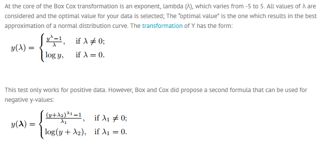
A Box Cox transformation is a way to transform non-normal dependent variables into a normal shape. Normality is an important assumption for many statistical techniques (for example when doing a linear regression, we assume that the errors are normally distributed); if your data isn’t normal, applying a Box-Cox means that you are able to run a broader number of tests.

https://www.statisticshowto.datasciencecentral.com/box-cox-transformation/

Application in R: https://www.youtube.com/watch?v=vGOpEpjz2Ks