Deep Learning
Introduction
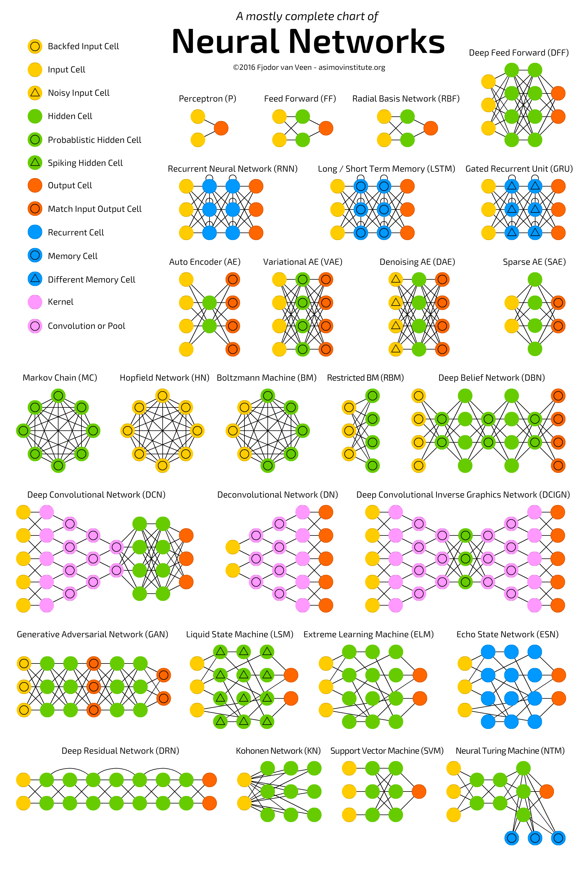
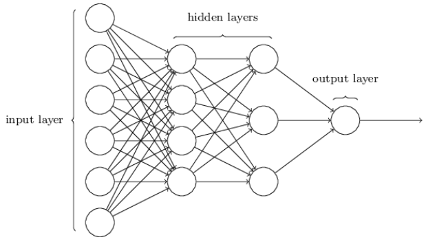
The different “beasts” in deep learning:
Deep learning is performing a universal function approximation. Provided that we have enough data, we can approximate any function.
Good general introduction links:
Intro to DL by playing, for both classification and regression: http://playground.tensorflow.org/
https://towardsdatascience.com/a-weird-introduction-to-deep-learning-7828803693b0
http://neuralnetworksanddeeplearning.com/chap1.html (Free online book)
General intro: https://towardsdatascience.com/deep-learning-with-python-703e26853820
Vanishing gradient: https://www.quora.com/What-is-the-vanishing-gradient-problem Vanishing gradient example: https://cs224d.stanford.edu/notebooks/vanishing_grad_example.html (exercise of clustering)
terminology: https://towardsdatascience.com/epoch-vs-iterations-vs-batch-size-4dfb9c7ce9c9
Terminology
epoch: One Epoch is when an ENTIRE dataset is passed forward and backward through the neural network only ONCE. We need indeed more than one epoch in order the optimizer (SGD or else) to update the weights of the net. One such iteration is not enough.
batch: the batch is a subset of the total dataset. The bacth size is the number of training examples present in a single batch. The total dataset is often divided into batches because it can sometimes be impossible to load the entire dataset in the neural net at once.
iterations: the iterations is the number of batches needed to complete one epoch. Note: The number of batches is equal to number of iterations for one epoch.
Let’s say we have dataset = 2000 training examples that we are going to use . We can divide the dataset of 2000 examples into batches of 500 then it will take 4 iterations to complete 1 epoch.
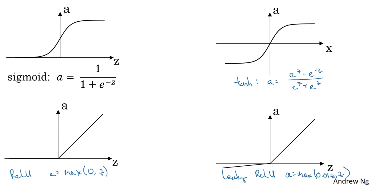
Activation functions
An activation function is a mapping of summed weighted input to the output of the neuron. It is called an activation/ transfer function because it governs the inception at which the neuron is activated and the strength of the output signal. Mathematically,
Y = SUM (weight * input) + bias
We have many activation functions, out of which most used are relu, tanh, solfPlus.
Here is a list of most useful activation functions:
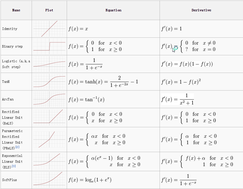
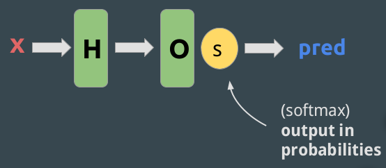
Softmax: The softmax function ensures that the output (most of time the last output, so the prediction) sums to one so that it can be interpreted as a probability.
ReLu
Leaky ReLu: almost same as ReLu, but in the negative side the values are not zero but decreasing slightly when going to the negative side. This gives better results than ReLu (Andrew Ng).
Why do we need non-linear activation functions? Why not to take the identity function? Simply because that would leave the model to be a simple linear operation, such as there are no hidden layers. And adding a sigmoid function at the end would make it equal as a simple logistic regression.

Back Propagation
The predicted value of the network is compared to the expected output, and an error is calculated using a function. This error is then propagated back within the whole network, one layer at a time, and the weights are updated according to the value that they contributed to the error. This clever bit of math is called the Back-Propagation algorithm. The process is repeated for all of the examples in your training data. One round of updating the network for the entire training dataset is called an epoch. A network may be trained for tens, hundreds or many thousands of epochs.

Loss / Cost functions
A loss (or cost) function, also known as an objective function, will specify the objective of minimizing loss/error, which our model will leverage to get the best performance over multiple epochsiterations. It again can be a string identifier to some pre-implemented loss functions like cross-entropy loss (classification) or mean squared error (regression) or it can be a custom loss function that we can develop. The loss/cost function is the measure of “how good” a neural network did for it’s given training input and the expected output. It also may depend on attributes such as weights and biases. A cost function is single-valued, not a vector because it rates how well the neural network performed as a whole. Using the Gradient Descent optimization algorithm, the weights are updated incrementally after each epoch.
Regression: mean_squared_error
Classification: categorical_crossentropy (lower score is better)
The full list for Keras is here: https://keras.io/losses/
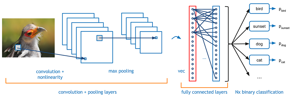
Convolutional Neural Networks (CNN)
The first few conv layers extract features like edges. The deeper conv layers extract complicated features like face, digits etc, that is the object of interest. This statement is an overgeneralization, but on a broader level this is true.
Here is a list of image classification datasets: https://dataturks.com/projects/Trending?type=IMAGE_CLASSIFICATION
Here is from scratch CNN (only Numpy needed): https://www.kdnuggets.com/2018/04/building-convolutional-neural-network-numpy-scratch.html
Convolution
On the other hand, Deep Learning simplifies the process of feature extraction through the process of convolution. Convolution is a mathematical operation, which maps out an energy function, which is a measure of similarity between two signals, or in our case images. So, when we use a blue filter and convolve it with white light, the resultant energy spectrum is that of blue light. Hence, the convolution of white light with a blue filter results in blue light. Hence term Convolutional Neural Networks, where feature extraction is done via the process of convolution.
Pooling
Pooling is a sub-sampling technique. The use of pooling is to reduce the dimension of the input image after getting convolved. There are two types, max pooling, and average pooling.

Batch Normalization
We add this layer initially, to normalize all the features. Technically, batch normalization normalizes the output of a previous activation layer(initially, input layer) by subtracting the batch mean and dividing by the batch standard deviation. This makes the model more robust and learns effectively. Intuitively, we are preventing overfitting!
Dropout
This is another regularization technique that was used before Batch Norm. The way this works is, the weights are randomly juggled around by very small amounts… the model ends up learning variations and again prevents overfitting. Individual nodes are either dropped out of the net with probability 1-p or kept with probability p so that a reduced network is left; incoming and outgoing edges to a dropped-out node are also removed.

Note on dropout:
Zero-Padding
This helps prevent dimensionality loss, during convolution. Thus, for very deep networks, we usually prefer this. The zeros don’t add to the energy quotient during the convolution and help maintain dimensionality at a required level.
Fully Connected Networks, or MultiPerceptron
The output from the convolutional layers represents high-level features in the data. While that output could be flattened and connected to the output layer, adding a fully-connected layer is a way of learning non-linear combinations of these features. Essentially the convolutional layers are providing a meaningful, low-dimensional, and somewhat invariant feature space and the fully-connected layer is learning a nonlinear function induced by the activation functions, in that space. Similar to an artificial neural network architecture.
Somewhat confusingly, and for historical reasons, such multiple layer networks are sometimes called multilayer perceptrons or MLPs, despite being made up of sigmoid neurons, not perceptrons.
Keras
Keras is a high-level Deep Learning framework for Python, which is capable of running on top of both Theano and Tensorflow. Keras allows us to use the constructs offered by Tensorflow and Theano in a much more intuitive and easy-to-use way without writing excess boilerplate code for building neural network based models.

This Cheatsheet is taken from DataCamp.
Install: on top of tensorflow: http://inmachineswetrust.com/posts/deep-learning-setup/
Loss functions
A loss function, also known as an objective function, will specify the objective of minimizing loss/error, which our model will leverage to get the best performance over multiple epochsiterations. It again can be a string identifier to some pre-implemented loss functions like cross-entropy loss (classification) or mean squared error (regression) or it can be a custom loss function that we can develop.
Regression: mean_squared_error
Classification: categorical_crossentropy (lower score is better)
The full list for Keras is here: https://keras.io/losses/
Optimizers
The role of the optimizer is to find the weights parameters that minimize the loss function.
One could use a simple Gradient Descent algorithm, but experience shows that it can be very long before reaching the Global/Local minimum. The Stochastic Gradient Descent (SGD) was introduced to reduce the time of convergence, still keeping an acceptable accuracy. Stochastic gradient descent maintains a single learning rate (termed alpha) for all weight updates and the learning rate does not change during training.
Three main variants of the SGD are available:
Adaptive Gradient Algorithm (AdaGrad) that maintains a per-parameter learning rate that improves performance on problems with sparse gradients (e.g. natural language and computer vision problems).
Root Mean Square Propagation (RMSProp) that also maintains per-parameter learning rates that are adapted based on the average of recent magnitudes of the gradients for the weight (e.g. how quickly it is changing). This means the algorithm does well on online and non-stationary problems (e.g. noisy).
Adam (the prefered one as to 2018, see here for a discussion: see https://machinelearningmastery.com/adam-optimization-algorithm-for-deep-learning/. ):
Why Adam?
Adam combines the best properties of the AdaGrad and RMSProp algorithms to provide an optimization algorithm that can handle sparse gradients on noisy problems.
Adam is relatively easy to configure where the default configuration parameters do well on most problems.
Instead of adapting the parameter learning rates based on the average first moment (the mean) as in RMSProp, Adam also makes use of the average of the second moments of the gradients (the uncentered variance).
Intro to Adam: https://machinelearningmastery.com/adam-optimization-algorithm-for-deep-learning/
For a thorough review, see http://ruder.io/optimizing-gradient-descent/
Nice post: https://medium.com/@nishantnikhil/adam-optimizer-notes-ddac4fd7218
The initial paper: https://arxiv.org/pdf/1412.6980.pdf
For an intro to SGD: http://neuralnetworksanddeeplearning.com/chap1.html and associated code: https://github.com/mnielsen/neural-networks-and-deep-learning/blob/master/src/network.py
comparison of optimizers: https://shaoanlu.wordpress.com/2017/05/29/sgd-all-which-one-is-the-best-optimizer-dogs-vs-cats-toy-experiment/
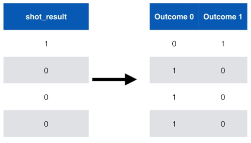
Conversion the label to categorical: One-Hot-Encoding
The OHE is used to convert the labels to categorical columns, one column per category, as seen here:
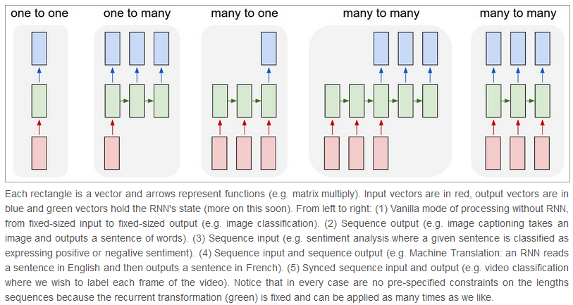
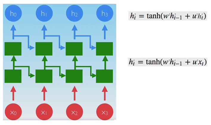
RNN: Recurrent Neural Networks
In RNNs, connections form a cycle: they are able to retain state from one iteration to the next by using their own input for the next step.
Here are the different types of RNNs:
Here is the vanilla RNN:
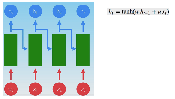
w, u weights do not depend on t: same weights at all times.
Deep networks can be built by stacking recurrent units onto one another:
RNN scheme is short term; it does not have a “memory” for far-past events.
Also, RNN suffers from vanishing gradients problem.
Good links: https://www.deeplearningbook.org/contents/rnn.html
An RNN from scratch in Numpy ONLY (great): https://www.analyticsvidhya.com/blog/2019/01/fundamentals-deep-learning-recurrent-neural-networks-scratch-python/?utm_source=linkedin.com&utm_medium=social
LSTM: Long Short-Term Memory
Here is the comparison of RNN vs LSTM

Here are details of the LSTM scheme:


Good links:
http://colah.github.io/posts/2015-08-Understanding-LSTMs/
http://adventuresinmachinelearning.com/recurrent-neural-networks-lstm-tutorial-tensorflow/
Post with Keras example: https://www.analyticsvidhya.com/blog/2017/12/fundamentals-of-deep-learning-introduction-to-lstm/
GRU (Gated Recurrent Unit): variant of LSTM
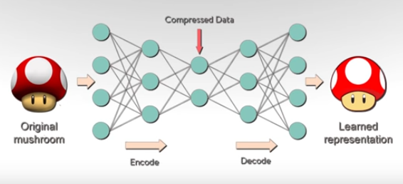
Autoencoders
Principle:
Links:
https://machinelearningmastery.com/encoder-decoder-long-short-term-memory-networks/
https://machinelearningmastery.com/develop-encoder-decoder-model-sequence-sequence-prediction-keras/
https://machinelearningmastery.com/define-encoder-decoder-sequence-sequence-model-neural-machine-translation-keras/ (more sequence to sequence)
http://rickyhan.com/jekyll/update/2017/09/14/autoencoders.html
https://github.com/keras-team/keras/issues/1029
https://github.com/keras-team/keras/issues/5203 #!!!
https://keras.io/layers/wrappers/
https://blog.keras.io/building-autoencoders-in-keras.html
https://machinelearningmastery.com/lstm-autoencoders/
Autoencoder with CNN: https://machinelearningmastery.com/how-to-develop-convolutional-neural-network-models-for-time-series-forecasting/
TimeDistributed layer: allows to apply a layer to every temporal slice of an input.
There are two key points to remember when using the TimeDistributed wrapper layer:
The input must be (at least) 3D. This often means that you will need to configure your last LSTM layer prior to your TimeDistributed wrapped Dense layer to return sequences (e.g. set the “return_sequences” argument to “True”).
The output will be 3D. This means that if your TimeDistributed wrapped Dense layer is your output layer and you are predicting a sequence, you will need to resize your y array into a 3D vector.
TimeDistributedDense applies a same Dense (fully-connected) operation to every timestep of a 3D tensor.
Here taken from https://github.com/keras-team/keras/issues/1029: But I think you still don’t catch the point. The most common scenario for using TimeDistributedDense is using a recurrent NN for tagging task.e.g. POS labeling or slot filling task.
In this kind of task: For each sample, the input is a sequence (a1,a2,a3,a4…aN) and the output is a sequence (b1,b2,b3,b4…bN) with the same length. bi could be viewed as the label of ai. Push a1 into a recurrent nn to get output b1. Than push a2 and the hidden output of a1 to get b2…
If you want to model this by Keras, you just need to used a TimeDistributedDense after a RNN or LSTM layer(with return_sequence=True) to make the cost function is calculated on all time-step output. If you don’t use TimeDistributedDense ans set the return_sequence of RNN=False, then the cost is calculated on the last time-step output and you could only get the last bN.
I am also new to Keras, but I am trying to use it to do sequence labeling and I find this could only be done by using TimeDistributedDense. If I make something wrong, please correct me.
Variational autoencoders
https://towardsdatascience.com/intuitively-understanding-variational-autoencoders-1bfe67eb5daf
https://medium.com/datadriveninvestor/variational-autoencoder-vae-d1cf436e1e8f
Variational Autoencoders (VAEs) have one fundamentally unique property that separates them from vanilla autoencoders, and it is this property that makes them so useful for generative modeling: their latent spaces are, by design, continuous, allowing easy random sampling and interpolation.
It achieves this by doing something that seems rather surprising at first: making its encoder not output an encoding vector of size n, rather, outputting two vectors of size n: a vector of means, μ, and another vector of standard deviations, σ.
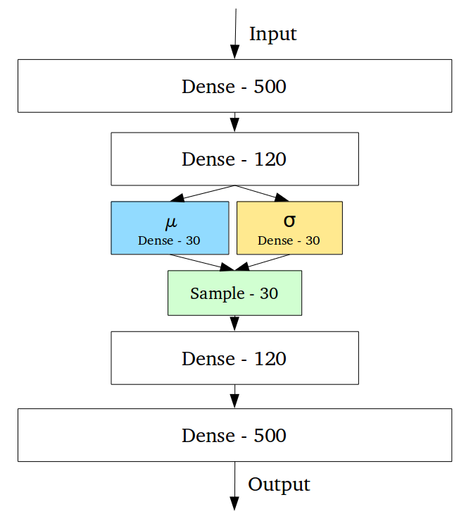
They form the parameters of a vector of random variables of length n, with the i th element of μ and σ being the mean and standard deviation of the i th random variable, X i, from which we sample, to obtain the sampled encoding which we pass onward to the decoder:
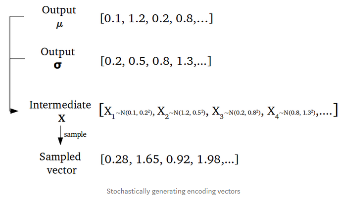
This stochastic generation means, that even for the same input, while the mean and standard deviations remain the same, the actual encoding will somewhat vary on every single pass simply due to sampling.
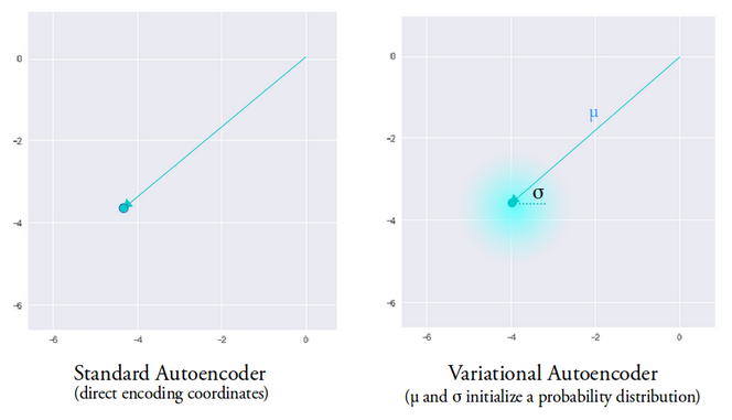
Intuitively, the mean vector controls where the encoding of an input should be centered around, while the standard deviation controls the “area”, how much from the mean the encoding can vary. As encodings are generated at random from anywhere inside the “circle” (the distribution), the decoder learns that not only is a single point in latent space referring to a sample of that class, but all nearby points refer to the same as well. This allows the decoder to not just decode single, specific encodings in the latent space (leaving the decodable latent space discontinuous), but ones that slightly vary too, as the decoder is exposed to a range of variations of the encoding of the same input during training
See also p 298 of “Deep learning in Python” from Chollet.
Genetic Algorithm hyperparameters tuning
Problem: the discovery of the best hyperparameters of a neural network is very time consuming, especially when it is done brute force. Here, we try to improve upon the brute force method by applying a genetic algorithm to evolve a network with the goal of achieving optimal hyperparameters in a fraction the time of a brute force search.
It is said that a 80% time saving can be obtained: https://blog.coast.ai/lets-evolve-a-neural-network-with-a-genetic-algorithm-code-included-8809bece164 (assuming best parameters are found…)
What’s a genetic algorithm? Genetic algorithms are commonly used to generate high-quality solutions to optimization and search problems by relying on bio-inspired operators such as mutation, crossover and selection. — Wikipedia (See here: https://lethain.com/genetic-algorithms-cool-name-damn-simple/)
See even simpler example here, based on Numpy only: https://www.kdnuggets.com/2018/07/genetic-algorithm-implementation-python.html
First: how do genetic algorithms work? At its core, a genetic algorithm…
Creates a population of (randomly generated) members
Scores each member of the population based on some goal. This score is called a fitness function.
Selects and breeds the best members of the population to produce more like them
Mutates some members randomly to attempt to find even better candidates
Kills off the rest (survival of the fittest and all), and
Repeats from step 2. Each iteration through these steps is called a generation.
Repeat this process enough times and you should be left with the very best possible members of a population.
See https://github.com/harvitronix/neural-network-genetic-algorithm for a code intro.
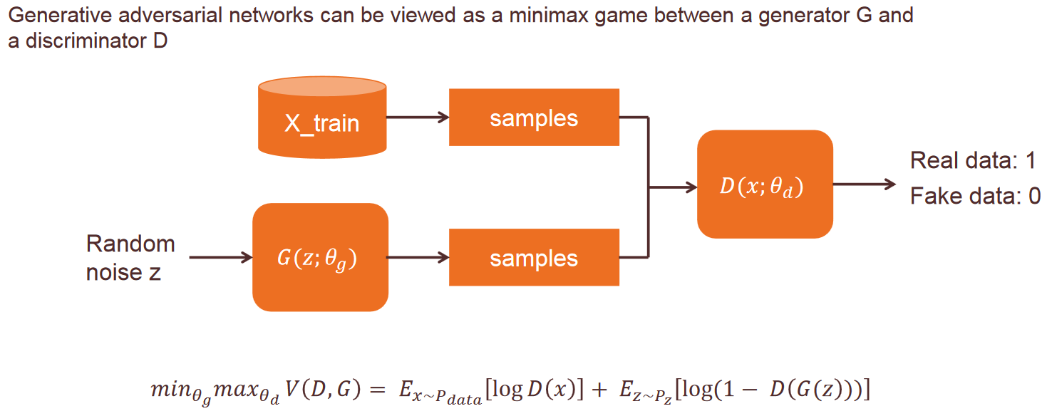
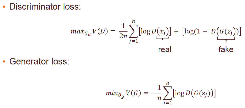
GAN: Generative Adversarial Networks
GAN is a family of Neural Network (NN) models that have two or more NN components (Generator/Discriminator) competing adversarially with each other that result in component NNs get better over time.
The models play two distinct (literally, adversarial) roles. Given some real data set R, G is the generator, trying to create fake data that looks just like the genuine data, while D is the discriminator, getting data from either the real set or G and labeling the difference. Goodfellow’s metaphor (and a fine one it is) was that G was like a team of forgers trying to match real paintings with their output, while D was the team of detectives trying to tell the difference. (Except that in this case, the forgers G never get to see the original data — only the judgments of D. They’re like blind forgers.)
Here is the metaphor of Ian Goodfellow:
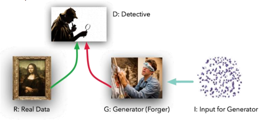
R: The original, genuine data set
I: The random noise that goes into the generator as a source of entropy
G: The generator which tries to copy/mimic the original data set
D: The discriminator which tries to tell apart G’s output from R
The actual ‘training’ loop where we teach G to trick D and D to beware G.
The GAN can be seen as a minmax game:
GANs can be used for anomaly detection:

Simple NN examples
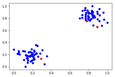
CLASSIFICATION: Example making new class predictions for a classification problem
from keras.models import Sequential
from keras.layers import Dense
from sklearn.datasets.samples_generator import make_blobs
from sklearn.preprocessing import MinMaxScaler

# generate 2d classification dataset
X, y = make_blobs(n_samples=100, centers=2, n_features=2, random_state=1)
scalar = MinMaxScaler()
scalar.fit(X)
X = scalar.transform(X)

# define and fit the final model
model = Sequential()
model.add(Dense(4, input_dim=2, activation='relu'))
model.add(Dense(4, activation='relu'))
model.add(Dense(1, activation='sigmoid'))
model.compile(loss='binary_crossentropy', optimizer='adam')
model.fit(X, y, epochs=500, verbose=0)

# new instances where we do not know the answer
Xnew, _ = make_blobs(n_samples=3, centers=2, n_features=2, random_state=1)
Xnew = scalar.transform(Xnew)
# make a prediction
ynew = model.predict_classes(Xnew)
# show the inputs and predicted outputs
for i in range(len(Xnew)):
    print("X=%s, Predicted=%s" % (Xnew[i], ynew[i]))

#Here just for visual check
import matplotlib.pyplot as plt
plt.plot(X[:,0],X[:,1],'bo')
plt.plot(Xnew[:,0],Xnew[:,1],'ro')
plt.show()

#output:
X=[0.89337759 0.65864154], Predicted=[0]
X=[0.29097707 0.12978982], Predicted=[1]
X=[0.78082614 0.75391697], Predicted=[0]
Note: Another type of prediction you may wish to make is the probability of the data instance belonging to each class:
Same, use ynew = model.predict_proba(Xnew) in place of ynew = model.predict_classes(Xnew)
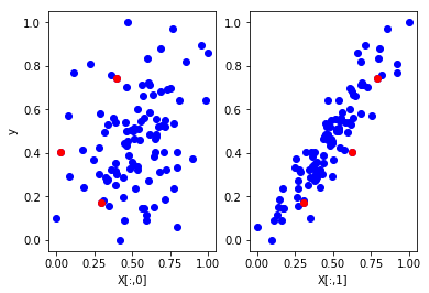
REGRESSION: Example of making predictions for a regression problem
from keras.models import Sequential
from keras.layers import Dense
from sklearn.datasets import make_regression
from sklearn.preprocessing import MinMaxScaler

# generate regression dataset
X, y = make_regression(n_samples=100, n_features=2, noise=0.1, random_state=1)
scalarX, scalarY = MinMaxScaler(), MinMaxScaler()
scalarX.fit(X)
scalarY.fit(y.reshape(100,1))
X = scalarX.transform(X)
y = scalarY.transform(y.reshape(100,1))

# define and fit the final model
model = Sequential()
model.add(Dense(4, input_dim=2, activation='relu'))
model.add(Dense(4, activation='relu'))
model.add(Dense(1, activation='linear'))
model.compile(loss='mse', optimizer='adam')
model.fit(X, y, epochs=1000, verbose=0)

# new instances where we do not know the answer
Xnew, a = make_regression(n_samples=3, n_features=2, noise=0.1, random_state=1)
Xnew = scalarX.transform(Xnew)

# make a prediction
ynew = model.predict(Xnew)
# show the inputs and predicted outputs
for i in range(len(Xnew)):
    print("X=%s, Predicted=%s" % (Xnew[i], ynew[i]))

#Here just for visual check
import matplotlib.pyplot as plt
ax=plt.subplot(1,2,1)
ax.plot(X[:,0],y,'bo')
ax.plot(Xnew[:,0],ynew,'ro')
ax.set_ylabel('y')
ax.set_xlabel('X[:,0]')
ax=plt.subplot(1,2,2)
ax.plot(X[:,1],y,'bo')
ax.plot(Xnew[:,1],ynew,'ro')
ax.set_xlabel('X[:,1]')
plt.show()

#output:
X=[0.29466096 0.30317302], Predicted=[0.17338811]
X=[0.39445118 0.79390858], Predicted=[0.7450506]
X=[0.02884127 0.6208843 ], Predicted=[0.4035678]
LSTM example
Taken from: https://machinelearningmastery.com/make-predictions-long-short-term-memory-models-keras/
from keras.models import Sequential
from keras.layers import Dense
from keras.layers import LSTM
from numpy import array
from keras.models import load_model

# return training data
def get_train():
    seq = [[0.0, 0.1], [0.1, 0.2], [0.2, 0.3], [0.3, 0.4], [0.4, 0.5]]
    seq = array(seq)
    X, y = seq[:, 0], seq[:, 1]
    X = X.reshape((len(X), 1, 1))
    return X, y

# define model
model = Sequential()
model.add(LSTM(10, input_shape=(1,1)))
model.add(Dense(1, activation='linear'))
# compile model
model.compile(loss='mse', optimizer='adam')
# fit model
X,y = get_train()
model.fit(X, y, epochs=300, shuffle=False, verbose=0)
# save model to single file
model.save('lstm_model.h5')
model.summary()
Then the model can be loaded again (from a different script in a different Python session) using the load_model() function.
from keras.models import load_model
# load model from single file
model = load_model('lstm_model.h5')
# make predictions
yhat = model.predict(X, verbose=0)
print(yhat)

#output
[[0.23529154]
 [0.27136612]
 [0.3086475 ]
 [0.34707576]
 [0.38658726]]
Again we can distinguish between predict(), predict_proba() and predict_classes():
Petastorm
#https://github.com/uber/petastorm #https://docs.azuredatabricks.net/applications/deep-learning/data-prep/petastorm.html #https://petastorm.readthedocs.io/en/latest/readme_include.html
Note that Petastorm produces Datasets that deliver data in batches that depends entirely on the Parquet files’ row group size. To control the batch size for training, it’s necessary to use Tensorflow’s unbatch() and batch() operations to re-batch the data into the right size. Also, note the small workaround that’s currently necessary to avoid a problem in reading Parquet files via Arrow in Petastorm.
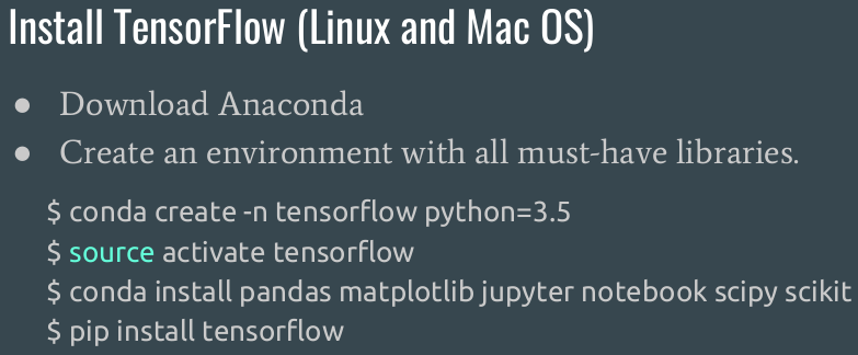
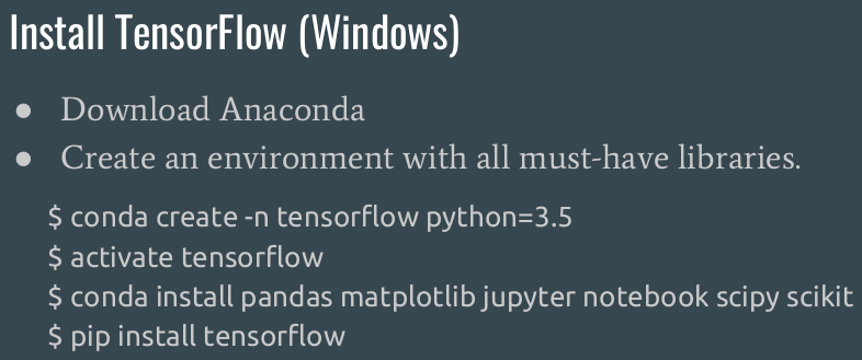
Tensorflow
Installation
Here is a cheatsheet taken from Tensorflow.
better: http://inmachineswetrust.com/posts/deep-learning-setup/
Here is a cheatsheet taken from Tensorflow.
Main Tensorflow outline
Here we will introduce the general flow of TensorFlow algorithms. Most recipes will follow this outline:
Import or generate datasets
Transform and normalize data: We will have to transform our data before we can use it, put in TensorFlow format. Most algorithms also expect normalized data. TensorFlow has built-in functions that can normalize the data for you as follows:
data = tf.nn.batch_norm_with_global_normalization(...)
Partition datasets into train, test, and validation sets
Set algorithm parameters (hyperparameters): Our algorithms usually have a set of parameters that we hold constant throughout the procedure. For example, this can be the number of iterations, the learning rate, or other fixed parameters of our choosing. It is considered good form to initialize these together so the user can easily find them, as follows:
learning_rate = 0.01
batch_size = 100
iterations = 1000
5. Initialize variables and placeholders: TensorFlow depends on knowing what it can and cannot modify. TensorFlow will modify/adjust the variables and weight/bias during optimization to minimize a loss function. To accomplish this, we feed in data through placeholders. We need to initialize both of these variables and placeholders with size and type, so that TensorFlow knows what to expect. See the following code:
a_var = tf.constant(42)
x_input = tf.placeholder(tf.float32, [None, input_size])
y_input = tf.placeholder(tf.float32, [None, num_classes])
Define the model structure: This is done by building a computational graph. TensorFlow chooses what operations and values must be the variables and placeholders to arrive at our model outcomes. For example, for a linear model:
y_pred = tf.add(tf.mul(x_input, weight_matrix), b_matrix)
Declare the loss functions: After defining the model, we must be able to evaluate the output. This is where we declare the loss function. The loss function is very important as it tells us how far off our predictions are from the actual values. Here is an example of loss function:
loss = tf.reduce_mean(tf.square(y_actual – y_pred))
Initialize and train the model: Now that we have everything in place, we need to create an instance of our graph, feed in the data through the placeholders, and let TensorFlow change the variables to better predict our training data. Here is one way to initialize the computational graph:
with tf.Session(graph=graph) as session:
  ...
  session.run(...)
  ...
Evaluate the model: Once we have built and trained the model, we should evaluate the model by looking at how well it does with new data through some specified criteria. We evaluate on the train and test set and these evaluations will allow us to see if the model is underfit or overfit.
Tune hyperparameters: Most of the time, we will want to go back and change some of the hyperparamters, based on the model performance. We then repeat the previous steps with different hyperparameters and evaluate the model on the validation set.
Deploy/predict new outcomes: It is also important to know how to make predictions on new, unseen, data. We can do this with all of our models, once we have them trained.
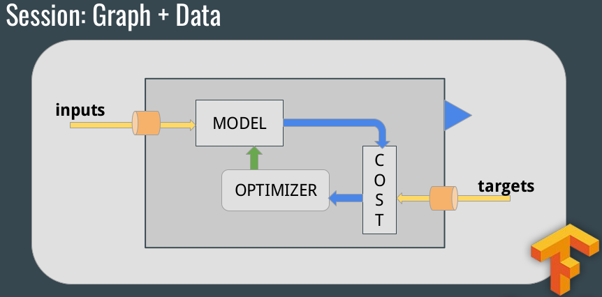
Graph, Session
The structure of TensorFlow programs is made of Graph and Session:
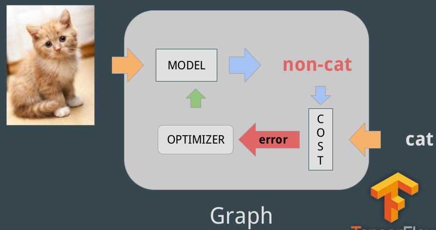
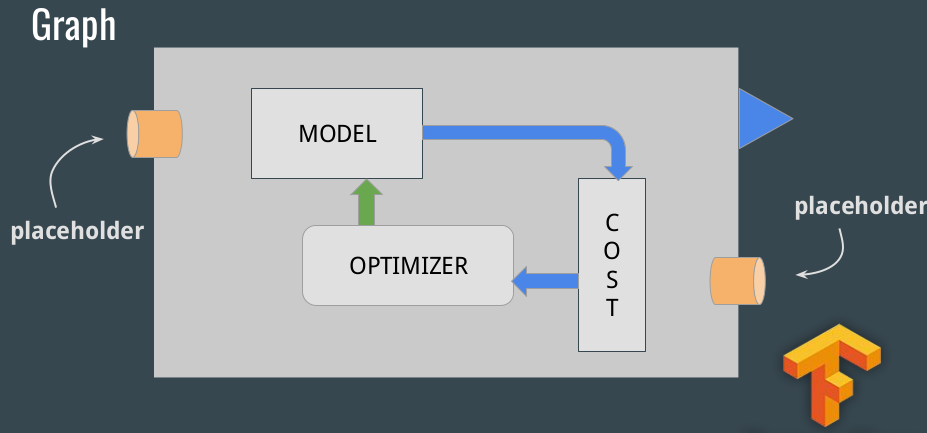
A graph is made of:
Placeholders: gates where we introduce example
Model: makes predictions. Set of variables and operations
Cost function: function that computes the model error
Optimizer: algorithm that optimizes the variables so the cost would be zero
Then the session is the Graph with the Data entered:
For example:
##### GRAPH #####
a = tf.placeholder(tf.int32)
b = tf.placeholder(tf.int32)
sum_graph = tf.add(a, b)
##### DATA #####
num1 = 3
num2 = 8
##### SESSION #####
with tf.Session() as sess:
  sum_outcome = sess.run(sum_graph, feed_dict={
  a: num1,
  b: num2
  })
  print("The sum of {} and {} is {}".format(num1,num2,sum_outcome))

The sum of 3 and 8 is 11
Data types
Matrices: here we create 5 matrices (2D arrays):
identity matrix
truncated normal distribution
an array with one fixed value
a uniform distribution array
an array conversion from Numpy
identity_matrix = tf.diag([1.0, 1.0, 1.0])
A = tf.truncated_normal([2, 3]) #or A = tf.truncated_normal([row_dim, col_dim],mean=0.0, stddev=1.0)
B = tf.fill([2,3], 5.0)
C = tf.random_uniform([3,2])
D = tf.convert_to_tensor(np.array([[1., 2., 3.],[-3., -7.,-1.],[0., 5., -2.]]))
print(sess.run(identity_matrix))
[[ 1.  0.  0.]
 [ 0.  1.  0.]
 [ 0.  0.  1.]]
print(sess.run(A))
[[ 0.96751703  0.11397751 -0.3438891 ]
 [-0.10132604 -0.8432678   0.29810596]]
print(sess.run(B))
[[ 5.  5.  5.]
 [ 5.  5.  5.]]
print(sess.run(C))
[[ 0.33184157  0.08907614]
 [ 0.53189191  0.67605299]
 [ 0.95889051  0.67061249]]
print(sess.run(D))
[[ 1.  2.  3.]
 [-3. -7. -1.]
 [ 0.  5. -2.]]
And for +,-,*, transposition, Determinant, Inverse operations:
print(sess.run(A+B))
[[ 4.61596632  5.39771316  4.4325695 ]
 [ 3.26702736  5.14477345  4.98265553]]
print(sess.run(B-B))
[[ 0.  0.  0.]
 [ 0.  0.  0.]]
print(sess.run(tf.matmul(B, identity_matrix)))
[[ 5.  5.  5.]
 [ 5.  5.  5.]]
print(sess.run(tf.transpose(C)))
[[ 0.67124544  0.26766731  0.99068872]
 [ 0.25006068  0.86560275  0.58411312]]
print(sess.run(tf.matrix_determinant(D)))
-38.0
print(sess.run(tf.matrix_inverse(D)))
[[-0.5        -0.5        -0.5       ]
 [ 0.15789474  0.05263158  0.21052632]
 [ 0.39473684  0.13157895  0.02631579]]
Eigenvalues and Eigenvectors:
print(sess.run(tf.self_adjoint_eig(D))
[[-10.65907521  -0.22750691   2.88658212]
 [  0.21749542   0.63250104  -0.74339638]
 [  0.84526515   0.2587998    0.46749277]
 [ -0.4880805    0.73004459   0.47834331]]
(The function self_adjoint_eig() outputs the eigenvalues in the first row and the subsequent vectors in the remaining vectors.)
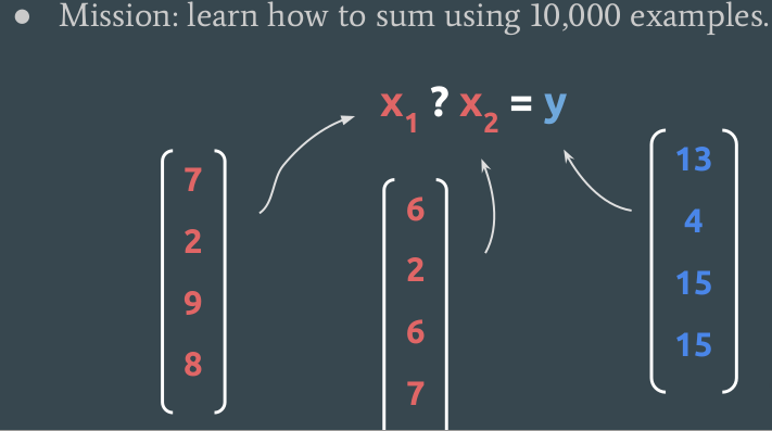
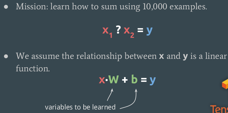
Regression
Here is a simple example of a regression exercise: let’s “learn” to a machine how to sum numbers! We give inputs and outputs, and it has to infer how to sum.
#Example taken from https://github.com/alesolano/mastering_tensorflow
We will use a linear model, with a weight matrix and a bias vector.
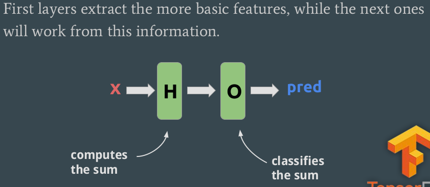
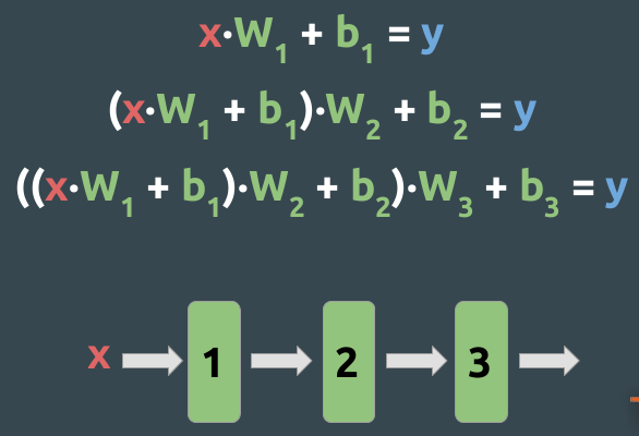
We could use different layers. The first ones are hidden, the last one is the output.
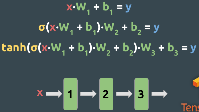
We could even put non-linear functions in the hidden layers:
Here is the full code for this exercise: this example script.
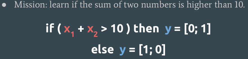
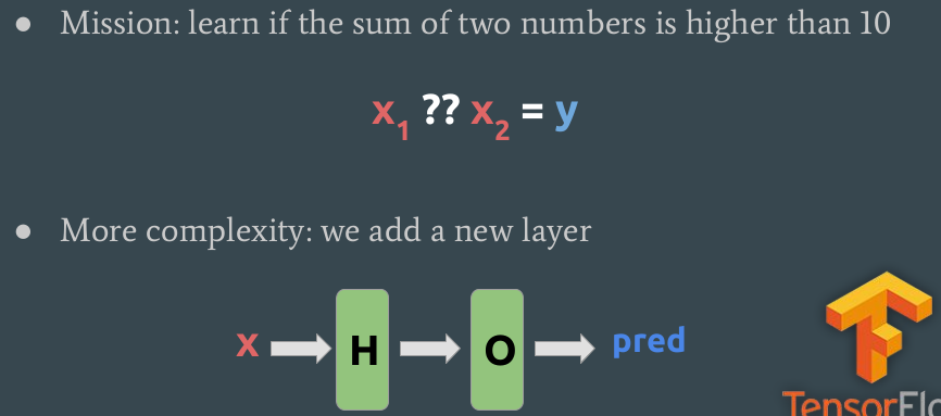
Classification
Exercise: let’s try to classify sums of 2 numbers, above 10 or not.
#Example taken from https://github.com/alesolano/mastering_tensorflow